
Experimental observations and posterior updating
Source:vignettes/experimental-observations-and-posterior-updating.Rmd
experimental-observations-and-posterior-updating.RmdPOWERUP predictions can be updated with experimental observations when both describe the same response on a comparable scale:
Prediction distributions -> Experimental observations -> Posterior distributions
prepare_powerup_observations() supports summarized
measurements and raw barcode counts.
Start with prediction distributions
After adding predictions to fitted models, request the long output
from summarize_predictions():
predictions <- summarize_predictions(models, format = "long")For posterior updating, the important columns are:
| Column | Meaning |
|---|---|
sample |
Prediction sample identifier |
perturbation |
Modeled perturbation |
pred_mean |
Predicted response mean |
pred_sd |
Prediction SD |
response_cutoff |
Cutoff defining the target event |
decreasing |
Whether the target event is at or below the cutoff |
calculate_powerup_posteriors() requires these six
columns and one unique row per sample-perturbation pair. The long
prediction table also includes prediction intervals and prior
target-event probabilities for interpretation.
For the compact example below, we will use three prediction distributions with the same required columns:
Option 1: summarized measurements
Use mode = "measurements" when an experiment has already
been summarized as a response estimate with uncertainty.
Required table
With the default column names, the input must look like this:
| sample | perturbation | value | sd |
|---|---|---|---|
| sample_a_exp | CTNNB1 | 0.91 | 0.06 |
| sample_a_exp | ERBB2 | 0.42 | 0.10 |
| sample_a_exp | FGFR1 | 0.18 | 0.08 |
The columns are:
-
sample: experimental sample identifier; -
perturbation: perturbation corresponding to the POWERUP model; -
value: observed response mean; -
sd: positive finite SD describing uncertainty in that observation.
There must be exactly one selected row for each sample-perturbation
pair. Custom column names can be supplied with sample_col,
perturbation_col, measurement_value_col, and
measurement_sd_col. If one table contains several
measurement types, use measurement_type_col together with
measurement_type to select one.
measurements <- data.frame(
  sample = c("sample_a_exp", "sample_a_exp", "sample_a_exp"),
  perturbation = c("CTNNB1", "ERBB2", "FGFR1"),
  value = c(0.91, 0.42, 0.18),
  sd = c(0.06, 0.10, 0.08)
)

observations <- prepare_powerup_observations(
  mode = "measurements",
  observations = measurements
)

observations
## # A tibble: 3 × 4
## sample perturbation observation_mean observation_sd
## <chr> <chr> <dbl> <dbl>
## 1 sample_a_exp CTNNB1 0.91 0.06
## 2 sample_a_exp ERBB2 0.42 0.1
## 3 sample_a_exp FGFR1 0.18 0.08The result contains the four columns needed for posterior updating:
sample, perturbation,
observation_mean, and observation_sd.
Option 2: raw barcode counts
Use mode = "barcode_counts" when starting from
replicate-level CRISPR barcode counts. POWERUP processes guide counts,
maps guides to targets, calibrates target-level measurements using
controls, and estimates observation uncertainty by hierarchical
bootstrap.
Barcode-count table
The counts table requires at least two barcode rows and exactly one
row per unique construct_barcode. An optional
construct_id column may also be present. All remaining
columns used in the analysis are sample count columns containing finite,
non-negative counts, and each sample used in the analysis must have a
non-zero total count.
| construct_barcode | construct_id | sample_a_T0_R1 | sample_a_T0_R2 | sample_a_T1_R1 | sample_a_T1_R2 |
|---|---|---|---|---|---|
| barcode_001 | guide_001 | 421 | 398 | 176 | 191 |
| barcode_002 | guide_002 | 305 | 322 | 298 | 281 |
| barcode_003 | guide_003 | 517 | 490 | 82 | 91 |
Sample names may end in T<number> for timepoint
and R<number> for replicate. POWERUP parses these
suffixes from the right, so underscores inside the base sample name are
preserved. For example:
parse_powerup_barcode_sample_names(c(
  "sample_a_T0_R1",
  "sample_a_T1_R2"
))
## # A tibble: 2 × 5
## raw_sample base_sample sample timepoint replicate
## <chr> <chr> <chr> <chr> <chr>
## 1 sample_a_T0_R1 sample_a sample_a_T0 T0 R1
## 2 sample_a_T1_R2 sample_a sample_a_T1 T1 R2analysis_samples uses the canonical sample name without
an R# suffix. sample_reference_map is a named
character vector whose names are base samples without T# or
R# suffixes and whose values are canonical reference
samples without an R# suffix:
analysis_samples = "sample_a_T1"
sample_reference_map = c(sample_a = "sample_a_T0")
Guide-reference table
The guide reference requires construct_barcode and
gene_symbol. gene_id is optional.
| construct_barcode | gene_symbol | gene_id |
|---|---|---|
| barcode_001 | CTNNB1 | 1499 |
| barcode_002 | ERBB2 | 2064 |
| barcode_003 | FGFR1 | 2260 |
The barcode identifiers must match those in the counts table.
positive_controls and negative_controls are
character vectors of perturbation names matching target names in the
guide reference after processing. Calibration requires matched targets
from both control classes and at least four control-target rows per
replicate, so multiple positive and negative controls should normally be
supplied.
The small example below uses two guides each for two positive controls, two negative controls, and one target. Two intergenic guides provide guide-level negative controls. The low-count filter is disabled only to keep the synthetic example small.
genes <- c(
  rep("POS1", 2), rep("POS2", 2), rep("NEG1", 2),
  rep("NEG2", 2), rep("GENE", 2),
  "ONE_INTERGENIC_SITE_A", "ONE_INTERGENIC_SITE_B"
)
barcodes <- paste0("BC", seq_along(genes))

barcode_counts <- data.frame(
  construct_barcode = barcodes,
  sample_a_T0 = c(100, 110, 120, 130, 140, 150, 160, 170, 180, 190, 200, 210),
  sample_a_T1_R1 = c(35, 40, 55, 60, 145, 155, 175, 185, 90, 95, 205, 215),
  sample_a_T1_R2 = c(40, 45, 50, 65, 150, 160, 180, 190, 85, 100, 210, 220)
)

guide_reference <- data.frame(
  construct_barcode = barcodes,
  gene_symbol = genes,
  gene_id = paste0("G", seq_along(genes))
)

barcode_observations <- prepare_powerup_observations(
  mode = "barcode_counts",
  counts = barcode_counts,
  guide_reference = guide_reference,
  analysis_samples = "sample_a_T1",
  sample_reference_map = c(sample_a = "sample_a_T0"),
  positive_controls = c("POS1", "POS2"),
  negative_controls = c("NEG1", "NEG2"),
  guide_negative_control_patterns = "ONE_INTERGENIC_SITE",
  guide_negative_control_fuzzy = TRUE,
  pseudogene_control_regex = "ONE_INTERGENIC_SITE",
  low_count_z_cutoff = -Inf,
  min_guides = 2L,
  bootstrap_repeats = 100L,
  bootstrap_seed = 1L
)
## [powerup][OBSERVATIONS_BOOTSTRAP] sample=sample_a_T1 replicates=2 targets=6 repeats=100## [powerup][OBSERVATIONS_BOOTSTRAP] sample=sample_a_T1 iteration=100/100## [powerup][OBSERVATIONS_BOOTSTRAP] sample=sample_a_T1 complete
barcode_observations[, c(
  "sample", "perturbation", "observation_mean", "observation_sd",
  "observation_bootstrap_prob_above_0_5", "observation_latent_sd",
  "observation_uncertainty_method"
)]
## # A tibble: 6 × 7
## sample perturbation observation_mean observation_sd observation_bootstra…¹
## <chr> <chr> <dbl> <dbl> <dbl>
## 1 sample_a_… GENE 1.00e+ 0 4.21e- 5 1
## 2 sample_a_… NEG1 8.72e-11 1.82e-10 0
## 3 sample_a_… NEG2 5.94e-12 1.31e-11 0
## 4 sample_a_… ONE_INTERGE… 2.16e-10 3.87e-10 0
## 5 sample_a_… POS1 1.00e+ 0 1.60e-11 1
## 6 sample_a_… POS2 1.00e+ 0 1.14e- 6 1
## # ℹ abbreviated name: ¹observation_bootstrap_prob_above_0_5
## # ℹ 2 more variables: observation_latent_sd <dbl>,
## # observation_uncertainty_method <chr>The default output again contains sample,
perturbation, observation_mean, and
observation_sd, along with barcode-analysis metadata. The
hierarchical bootstrap also records
observation_bootstrap_prob_above_0_5, the fraction of valid
bootstrap realizations whose control-calibrated probability is at least
0.5, and logit-scale bootstrap summaries.
observation_latent_sd exposes the directly estimated
logit-scale uncertainty used when
calculate_powerup_posteriors(..., response_transform = "logit")
is requested. You can set return_details = TRUE when the
intermediate guide-, target-, calibration-, and bootstrap-level tables
are needed.
By default, target z-score p-values use the two-sided standard-normal
distribution. Set target_pvalue_method = "empirical_null"
to compare each target z-score with a within-sample null generated by
repeatedly resampling negative-control guides and grouping them into
synthetic pseudogenes. The empirical null uses
bootstrap_repeats and bootstrap_seed,
empirical p-values use a finite-sample correction, and FDR is calculated
within each sample for either method.
Posterior updating assumes that the predictive prior and experimental observation describe the same underlying response on a comparable scale. Measurement mode requires a positive finite SD. In barcode-count mode, at least two analysis replicates are needed to estimate bootstrap uncertainty; a single replicate can be processed, but it does not provide the positive observation SD required for posterior updating. Positive and negative controls must both be represented for calibration.
Calculate posterior distributions
Prediction and observation rows are matched by sample
and perturbation. If the prediction and experimental sample
identifiers differ, provide a named sample_map from
prediction sample ID to observation sample ID:
posteriors <- calculate_powerup_posteriors(
  predictions_example,
  observations,
  sample_map = c("sample_a_prediction" = "sample_a_exp"),
  response_transform = "logit")

posteriors
## # A tibble: 3 × 23
## sample perturbation response_cutoff decreasing prior_mean prior_sd
## <chr> <chr> <dbl> <lgl> <dbl> <dbl>
## 1 sample_a_exp CTNNB1 0.5 FALSE 0.82 0.12
## 2 sample_a_exp ERBB2 0.5 FALSE 0.55 0.18
## 3 sample_a_exp FGFR1 0.5 FALSE 0.22 0.1
## # ℹ 17 more variables: prior_prob_target_event <dbl>, observation_mean <dbl>,
## # observation_sd <dbl>, posterior_mean <dbl>, posterior_sd <dbl>,
## # posterior_pi_lower_95 <dbl>, posterior_pi_upper_95 <dbl>,
## # posterior_prob_target_event <dbl>, posterior_status <chr>,
## # response_transform <chr>, response_cutoff_latent <dbl>,
## # prior_latent_mean <dbl>, prior_latent_sd <dbl>,
## # observation_latent_mean <dbl>, observation_latent_sd <dbl>, …For each matched pair, POWERUP performs inverse-variance weighting on
the scale selected by response_transform. A more precise
source contributes more strongly to the latent posterior. Returned
means, SDs, intervals, cutoffs, and plots remain on the original
biological response scale.
response_transform = "identity" is the default and
exactly preserves the original Gaussian-Gaussian update. Use
"logit" for responses constrained to (0, 1),
"log" or "log10" for strictly positive
responses such as concentration measurements, and
"identity" for outcomes such as z-scores or other
approximately unbounded continuous responses.
The main output columns are:
| Column | Meaning |
|---|---|
prior_mean, prior_sd
|
Predictive distribution before the experiment |
prior_prob_target_event |
Prior probability of satisfying the response cutoff |
observation_mean, observation_sd
|
Experimental distribution |
posterior_mean, posterior_sd
|
Updated response distribution |
posterior_pi_lower_95,
posterior_pi_upper_95
|
95% posterior interval |
posterior_prob_target_event |
Updated probability of satisfying the response cutoff |
posterior_status |
Whether the requested update was available |
response_transform |
Scale used for Gaussian evidence integration |
prior_latent_mean, prior_latent_sd
|
Predictive distribution on the integration scale |
observation_latent_mean,
observation_latent_sd
|
Experimental distribution on the integration scale |
posterior_latent_mean,
posterior_latent_sd
|
Posterior distribution on the integration scale |
The target event follows the model definition: when
decreasing = TRUE, it is P(y <= cutoff);
otherwise it is P(y >= cutoff). Because all supported
transformations are monotone increasing, the same event direction is
retained on the latent scale.
Visualize an update
plot_posterior() displays the predictive prior,
experimental observation, and posterior for one sample and perturbation.
Transformed updates are plotted as the corresponding transformed-normal
densities on the original response scale; for example, a logit update
remains on a 0-to-1 probability axis:
plot_posterior(
  posteriors,
  perturbation = "CTNNB1",
  sample = "sample_a_exp",
  fixed_axis = TRUE
)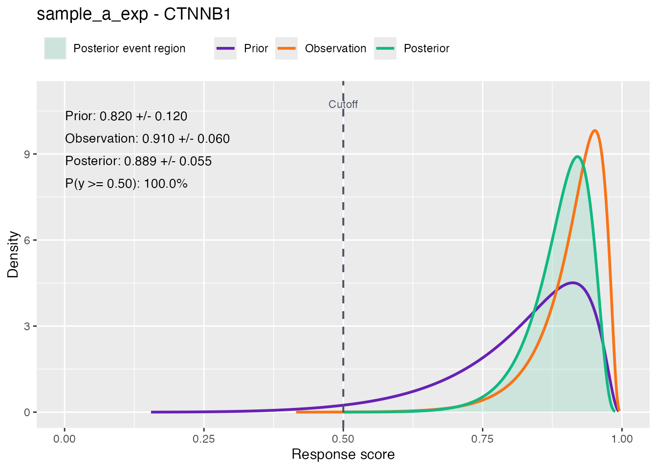
The shaded region represents the posterior probability assigned to the target event.
Next step
See Interpreting POWERUP results for guidance on model performance, prediction uncertainty, and posterior probabilities. For detailed SHAP interpretation, see Explaining POWERUP predictions.
Session information
## R version 4.4.2 (2024-10-31)
## Platform: aarch64-apple-darwin20
## Running under: macOS Sequoia 15.7.3
##
## Matrix products: default
## BLAS:   /Library/Frameworks/R.framework/Versions/4.4-arm64/Resources/lib/libRblas.0.dylib
## LAPACK: /Library/Frameworks/R.framework/Versions/4.4-arm64/Resources/lib/libRlapack.dylib;  LAPACK version 3.12.0
##
## locale:
## [1] en_US.UTF-8/en_US.UTF-8/en_US.UTF-8/C/en_US.UTF-8/en_US.UTF-8
##
## time zone: America/New_York
## tzcode source: internal
##
## attached base packages:
## [1] stats     graphics  grDevices utils     datasets  methods   base
##
## other attached packages:
## [1] powerup_1.0.117
##
## loaded via a namespace (and not attached):
##  [1] gtable_0.3.6      jsonlite_2.0.0    dplyr_1.1.4       compiler_4.4.2
##  [5] tidyselect_1.2.1  tidyr_1.3.1       jquerylib_0.1.4   systemfonts_1.2.2
##  [9] scales_1.3.0      textshaping_1.0.0 yaml_2.3.10       fastmap_1.2.0
## [13] ggplot2_3.5.1     R6_2.6.1          labeling_0.4.3    generics_0.1.3
## [17] knitr_1.50        htmlwidgets_1.6.4 tibble_3.3.0      desc_1.4.3
## [21] munsell_0.5.1     bslib_0.9.0       pillar_1.10.1     rlang_1.1.6
## [25] utf8_1.2.4        cachem_1.1.0      xfun_0.51         fs_1.6.5
## [29] sass_0.4.9        cli_3.6.5         pkgdown_2.2.0     withr_3.0.2
## [33] magrittr_2.0.3    digest_0.6.37     grid_4.4.2        lifecycle_1.0.4
## [37] vctrs_0.6.5       evaluate_1.0.3    glue_1.8.0        farver_2.1.2
## [41] ragg_1.5.1        colorspace_2.1-1  rmarkdown_2.29    purrr_1.1.0
## [45] tools_4.4.2       pkgconfig_2.0.3   htmltools_0.5.8.1